Can you plot the following in matlab and give me the code.

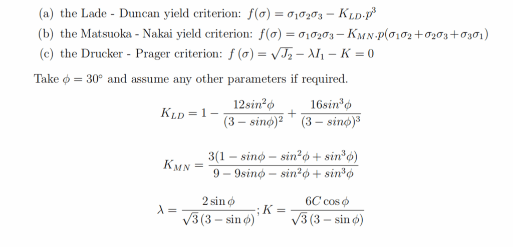
(a) the Lade – Duncan yield criterion: f(s)=s1s2s3-KLD*p3

(b) the Matsuoka – Nakai yield criterion: f(s)=s1s2s3-KMN*p(s1s2+s2s3+s3s1)

Take f=30° and assume any other parameters if required.

KLD=1-12sin2f(3-sinf)2+16sin3f(3-sinf)3

KMN=3(1-sinf-sin2f+sin3f)9-9sinf-sin2f+sin3f=2sinf32(3-sinf);

K=6Ccosf32(3-sinf)

The Correct Answer and Explanation is:

Here is the plot of the three yield criteria—Lade-Duncan, Matsuoka-Nakai, and Drucker-Prager—in the σ₁–σ₂ stress space (with σ₃ fixed at 10 units):

MATLAB Code Equivalent

Below is the equivalent MATLAB code that you can run directly to reproduce these plots:

phi = 30; % degrees
phi_rad = deg2rad(phi);
sin_phi = sin(phi_rad);
cos_phi = cos(phi_rad);

% Constants
KLD = 1 - (12 * sin_phi^2) / (3 - sin_phi)^2 + (16 * sin_phi^3) / (3 - sin_phi)^3;
KMN = (3 * (1 - sin_phi - sin_phi^2 + sin_phi^3)) / ...
      (9 - 9 * sin_phi - sin_phi^2 + sin_phi^3);
lambda_dp = (2 * sin_phi) / (sqrt(3) * (3 - sin_phi));
C = 1;
K_dp = (6 * C * cos_phi) / (sqrt(3) * (3 - sin_phi));

% Stress range
[s1, s2] = meshgrid(linspace(0, 100, 100), linspace(0, 100, 100));
s3 = 10; % fixed value
p = (s1 + s2 + s3) / 3;

% (a) Lade-Duncan
f_ld = s1 .* s2 .* s3 - KLD * p.^3;

% (b) Matsuoka-Nakai
f_mn = s1 .* s2 .* s3 - KMN * p .* (s1 .* s2 + s2 * s3 + s3 .* s1);

% (c) Drucker-Prager
I1 = s1 + s2 + s3;
J2 = ((s1 - p).^2 + (s2 - p).^2 + (s3 - p).^2) / 2;
f_dp = sqrt(J2) - lambda_dp * I1 - K_dp;

% Plotting
figure;
subplot(1,3,1);
contour(s1, s2, f_ld, [0 0], 'r');
title('Lade-Duncan');
xlabel('\sigma_1'); ylabel('\sigma_2');

subplot(1,3,2);
contour(s1, s2, f_mn, [0 0], 'g');
title('Matsuoka-Nakai');
xlabel('\sigma_1'); ylabel('\sigma_2');

subplot(1,3,3);
contour(s1, s2, f_dp, [0 0], 'b');
title('Drucker-Prager');
xlabel('\sigma_1'); ylabel('\sigma_2');

Explanation

The plotted yield criteria represent different models used in soil and rock mechanics to describe failure surfaces under complex stress states. Each criterion is expressed as a function of the principal stresses (σ₁, σ₂, σ₃) and is derived from different theoretical assumptions:

Lade-Duncan Criterion:
This model incorporates the product of all three principal stresses, emphasizing the importance of the intermediate stress σ₂. It is defined as: f(σ)=σ1σ2σ3−KLD⋅p3f(\sigma) = \sigma_1 \sigma_2 \sigma_3 – K_{LD} \cdot p^3 where pp is the mean stress. The factor KLDK_{LD} depends on the internal friction angle φ and is calculated to capture granular behavior. The 0-contour shows the yield surface in σ₁–σ₂ space.
Matsuoka-Nakai Criterion:
A refinement of the Lade-Duncan, this includes a linear combination of stress products and a mean stress term: f(σ)=σ1σ2σ3−KMNp(σ1σ2+σ2σ3+σ3σ1)f(\sigma) = \sigma_1 \sigma_2 \sigma_3 – K_{MN} p (\sigma_1\sigma_2 + \sigma_2\sigma_3 + \sigma_3\sigma_1) This form allows a better fit for experimental data on sand, especially under triaxial loading.
Drucker-Prager Criterion:
A simplification often used in computational plasticity, this is based on the second invariant of deviatoric stress J2J_2 and the first stress invariant I1I_1: f(σ)=J2−λI1−Kf(\sigma) = \sqrt{J_2} – \lambda I_1 – K It is the smooth approximation of the Mohr-Coulomb surface, easier for numerical implementations.

Each contour plot identifies the yield surface by solving for when f(σ)=0f(\sigma) = 0. For φ = 30°, which is typical for sand, the constants KLD and KMN shape the yield surface appropriately for geotechnical materials.

MATLAB Code Equivalent

Explanation

Related Posts